6. 데이터 시각화
1) 그래프 그리기
2) 그래프에 객체 추가하기
3) 지도 시각화: ggmap 패키지
1) 그래프 그리기
(1) ggplot( ) 함수: 그래프 기본 틀 만들기
- 그래프를 표현하는 좌표를 그리기 위한 함수로
* geom_로 시작하는 함수를 통해 각종 그래프를 추가하는 형태
- install.packages("ggplot2") 패키지 설치 필요
- library(ggplot2)
- ggplot(데이터 세트, aes(데이터 속성))
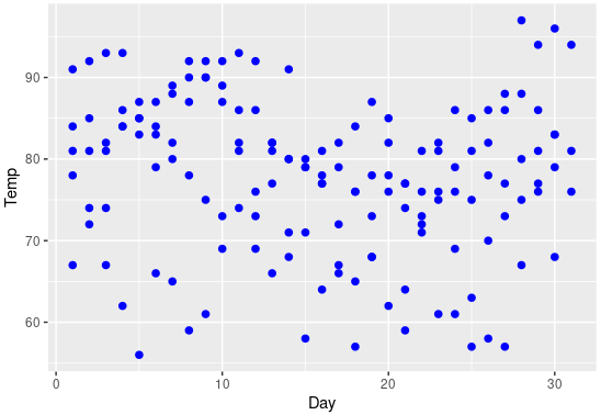
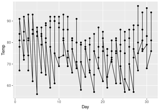
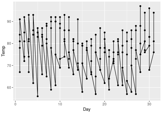
| 산점도 그리기 | 선 그래프 그리기 |
| geom_point( ) 함수 | geom_line( ) 함수 |
| > ggplot(airquality, aes(x=Day, y=Temp)) + geom_point(size=2, color="blue") | > ggplot(airquality, aes(x=Day, y=Temp)) + geom_line() + geom_point() |
 |
 |
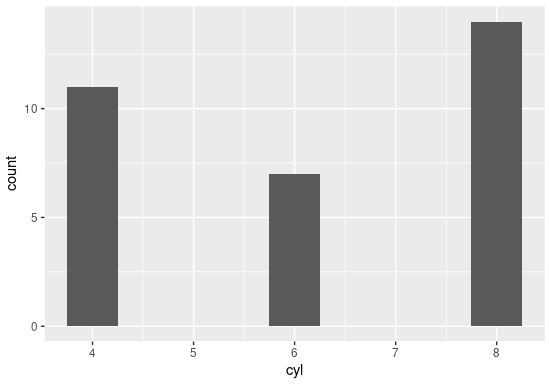
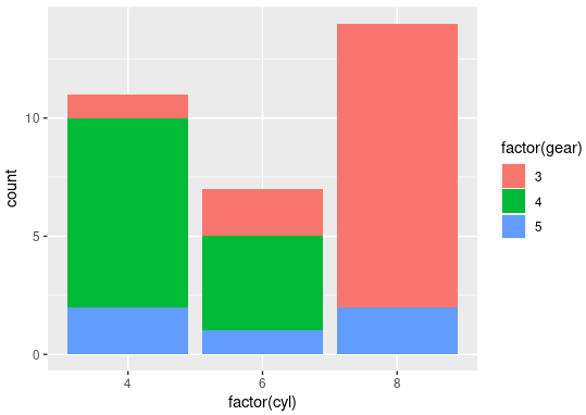
| 막대 그래프 그리기 | 누적 막대 그래프 그리기 |
| geom_bar( ) 함수 | geom_bar( aes() ) 함수 |
| > ggplot(mtcars, aes(x=cyl)) + geom_bar(width=0.5) | > ggplot(mtcars, aes(x=factor(cyl))) + geom_bar(aes(fill=factor(gear))) → factor 함수로 빈 범주를 제외함 → fill 함수로 gear 변수의 빈도가 색상으로 채워짐 |
 |
 |
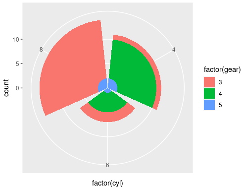
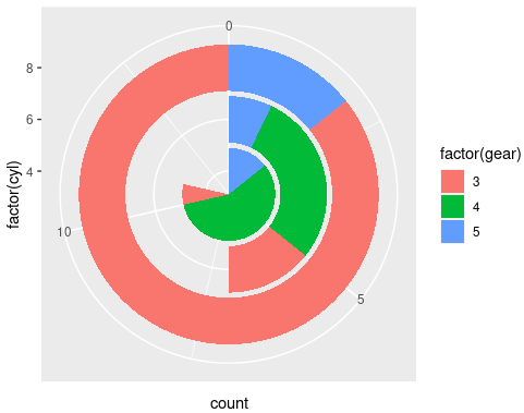
| 선버스트 차트 | 도넛 모양의 선버스트 차트 |
| coord_polar( ) 함수 | coord_polar(theta="y") 함수 |
| > ggplot(mtcars, aes(x=factor(cyl))) + geom_bar(aes(fill=factor(gear))) + coord_polar() | > ggplot(mtcars, aes(x=factor(cyl))) + geom_bar(aes(fill=factor(gear))) + coord_polar(theta="y") |
 |
 |
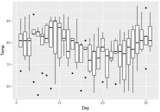
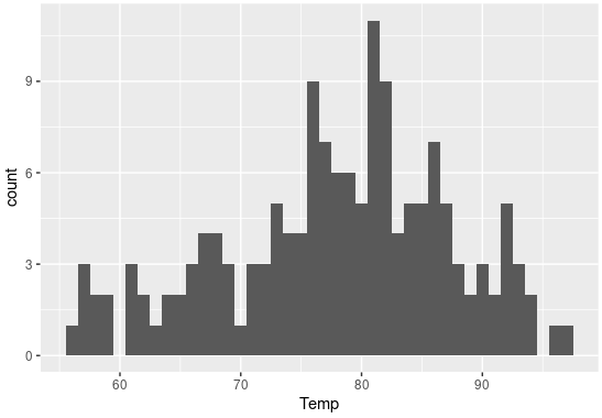
| 상자 그림 그리기 | 히스토그램 그리기 |
| geom_boxplot( ) 함수 | geom_histogram( ) 함수 |
| > ggplot(airquality, aes(x=Day, y=Temp, group=Day)) + geom_boxplot() | > ggplot(airquality, aes(Temp)) + geom_histogram(binwidth=1) |
 |
 |
2) 그래프에 객체 추가하기
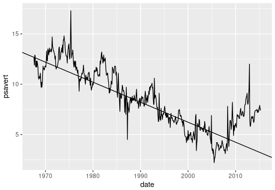
(1) 추세선 그리기
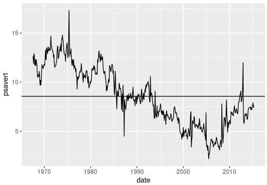
| 사선 그리기 | 평행선 그리기 | 수직선 그리기 |
| geom_abline(intercept=절편, slope=기울기) | geom_hline(yintercept=y절편) | geom_vline(xintercept=x절편) |
| > ggplot(economics, aes(x=date, y=psavert)) + geom_line() + geom_abline(intercept=12.18671, slope=-0.0005444) | > ggplot(economics, aes(x=date, y=psavert)) + geom_line() + geom_hline(yintercept=mean(economics$psavert)) | > ggplot(economics, aes(x=date, y=psavert)) + geom_line() + geom_vline(xintercept=as.Date("2005-07-01")) |
 |
 |
 |
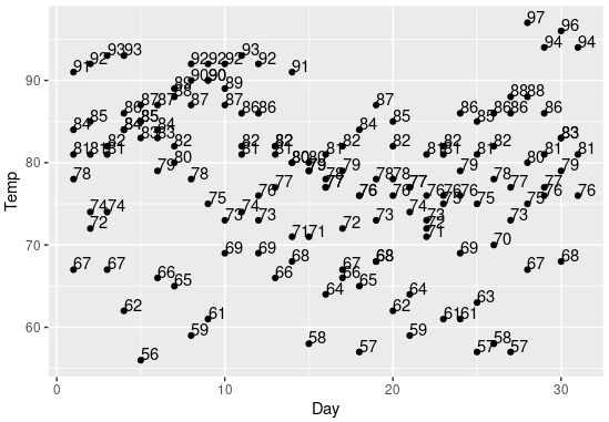
| 레이블 입력하기 |
| geom_text(aes(label=레이블, vjust=세로위치, hjust=가로위치) |
| > ggplot(airquality, aes(x=Day, y=Temp)) + geom_point() + geom_text(aes(label=Temp, vjust=0, hjust=0)) |
 |
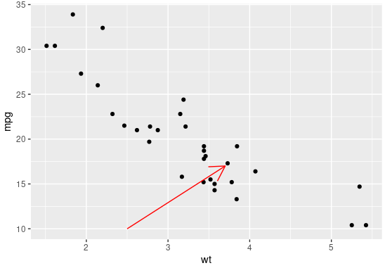
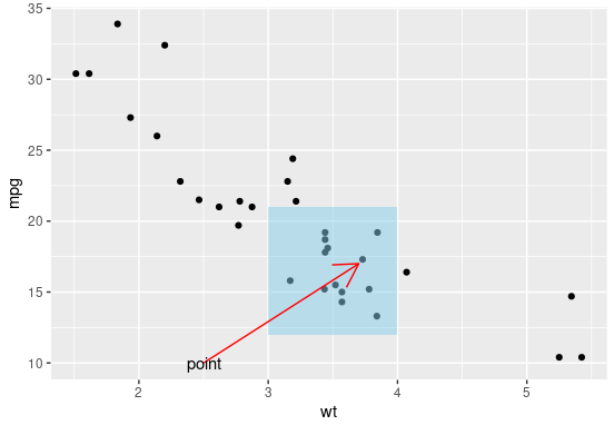
| 도형 그리기 | 화살표 그리기 | 텍스트 입력 |
| annotate("모양", xmin=x축시작, xmax=x축끝, ymin=y축시작, ymax=y축끝) | annotate("segment", x=x축시작, xend=x축끝, y=y축시작, yend=y축끝, arrow=arrow()) | annotate("text", x=x축위치, y=y축위치, label="텍스트내용") |
| > ggplot(mtcars, aes(x=wt, y=mpg)) + geom_point() + annotate("rect", xmin=3, xmax=4, ymin=12, ymax=21, alpha=0.5, fill="skyblue") | > ggplot(mtcars, aes(x=wt, y=mpg)) + geom_point() + annotate("segment", x=2.5, xend=3.7, y=10, yend=17, color="red", arrow=arrow()) | > ggplot(mtcars, aes(x=wt, y=mpg)) + geom_point() + annotate("text", x=2.5, y=10, label="point") |
 |
 |
 |
3) 지도 시각화: ggmap 패키지
(1) 구글 지도 API 키 발급
- 구글 지도 플랫폼 홈페이지(https://mapsplatform.google.com/) 접속
- 구글 클라우드 플랫폼 약관 동의, 결제 정보 입력, 사용 설정 설문조사 제출하면 API 키가 발급 완료됨
(2) ggmap 패키지
- 구글 지도 API 서비스를 활용하여 지도 시각화를 할 수 있는 패키지
- install.packages("ggmap") 패키지 설치 필요
- library(ggmap)
- register_google(key = "API 키"): 발급받은 구글 지도 API키 등록
- get_googlemap("지역명", maptype = "roadmap"): 설정한 위치를 지도로 가져오는 함수
- get_googlemap(c(lon=경도, lat=위도), maptype = "roadmap")
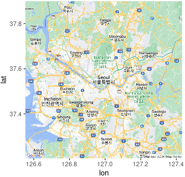
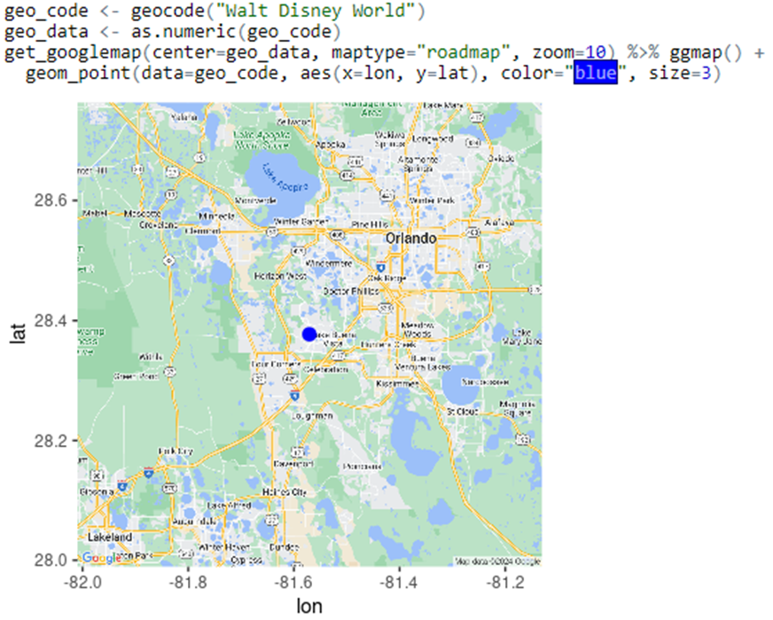
| 지도로 시각화 | 특정 위치의 경도 및 위도값 |
| ggmap( ) 함수 | geocode( ) 함수 |
| > gg_seoul <- get_googlemap("seoul", maptype="roadmap") > ggmap(gg_seoul) |
> geo_code <- enc2utf8("뉴욕") %>% geocode() > geo_data <- as.numeric(geo_code) > get_googlemap(center=geo_data, maptype="roadmap", zoom=13) %>% ggmap() + geom_point(data=geo_code, aes(x=geo_code$lon, y= geo_code$lat), color="red") |
 |
 |
* enc2utf8( ) 함수로 한글을 인코딩 함
6주차. 기본 미션
p288의 <좀 더 알아보기> 실습하고 결과 화면 캡처하기
> ggplot(airquality, aes(x=Day, y=Temp)) + geom_line() + geom_point()
6주차. 선택 미션
구글 API와 ggmap 패키지를 활용해서 원하는 장소의 지도를 불러온 후 결과 화면 인증하기
'혼공학습단 > 혼자 공부하는 R 데이터 분석' 카테고리의 다른 글
| [혼공R이] 12기 마무리하며♡ (0) | 2024.08.18 |
|---|---|
| [혼공R이] #7. 프로젝트로 실력 다지기 (0) | 2024.08.14 |
| [혼공R이] #5. 데이터 가공하기 (0) | 2024.08.05 |
| [혼공R이] #4. 데이터 다루기 (1) | 2024.07.22 |
| [혼공R이] #3. R 프로그래밍 익히기 (1) | 2024.07.20 |